
Symm. Cosmological Model in electromagnetic field…
A non static cylindrically symmetric cosmological model in presence of electromagnetic field
Abhishek Kumar Singh1. Dr. R.B.S. Yadav2.
Department of Mathematics Magadh University, Bodhgaya-824234,
1.1 Abstract :
The cylindrically symmetric models in presence of electromagnetic field play a significant role in understanding some essential feature of cosmological models. The occurrence of magnetic fields on a galactic scale is a well-established fact today, and its importance for a variety of astrophysical phenomena, interstellar spaces exhibit the presence of strong magnetic field and the magnatohydrodynamical processes in stars.
In this paper, considering the cylindrically symmetric metric of Marder [12], i.e, ds^2= α^2 (〖dt〗^2- 〖dx〗^2 )- β^2 〖dy〗^2- γ^2 〖dz〗^2
, where the metric potential α,β,γ are function of time t alone.We have constructed a non static spatially homogeneous Petrov type -I cosmological model assuming the energy momentum tensor to be that of a perfect fluid with an electromagnetic field and the four current is either zero or space like. For this we assume that, the space time is of degenerate Petrov type – I, being in y and z directions.
This requires that
The requirement that the conductivity be positive imposes an additional condition on the metric functions. Various physical and geometrical properties e.g. pressure, density, rotation scalar of expansion and components of shear tensor have been found. We have also discussed Doppler Effect and Newtonian analogue of force in the model. We have shown that when cosmological term ᴧ = 0 then in the absence of electromagnetic field, pressure and density becomes equal i.e. p=ρ and conversely.
1.2 Introduction :
The cylindrically symmetric cosmological models in presence of electromagnetic field play a significant role in understanding some essential feature of cosmological models [20, 37]. The occurrence of magnetic fields on a galactic scale is a well-established fact today, and its importance for a variety of astrophysical phenomena is generally acknowledged as pointed out by Zeldovich et.al [34]. Various researchers have paid their attention in obtaining the cosmological models in the presence of electromagnetic field in General Relativity [4, 18, 23]. Roy and Prakash [24] have studied the behaviour of magnetic field in the models of the universe. Before starting the work a general idea of magneto hydrodynamics is essential. Magnetohydynamics is the study of the motion of an electrically conducting field in the presence of a magnetic field. Electric currents induced in the fluid as a result of its motion modify the field; at the same time their flow in the magnetic field produces mechanical forces which modify the motion. Magnetohydrodynamics owes its peculiar interest and difficulty to the interaction between the field and the motion.
It is well known that galaxies and interstellar spaces exhibit the presence of strong magnetic field [35-36] which impart a sort of viscous effect in the fluid flow [6]. The magnetic field assumes an important role for the universe. The behaviour of the magnetic held of a star was investigated by Cowling [5] and Wrubel [31]. The important results obtained make possible the interpretation of magnatohydrodynamical processes in stars. When motions of stellar matter caused by the electromagnetic forces are taken into account, new properties may be revealed and the non-stability of the magneto hydro dynamical processes in stars may be studied. A cosmological model in the presence of magnetic field has been studied by Zeldovich [34] and later by Thorne [27], Shikin [25] also constructed a uniform axially symmetric solution (model) of Einstein Maxwell equations in the case of propagation by an ideal fluid in the presence of magnetic field directed along the axis of symmetry. Magnetic field in stellar bodies was also discussed by Monoghan [15]. Gravitationally collapse of a magnetic star was studied by Greenburg [10]. Jacobs [12-12a] has studied the behaviour of the general Bianchi- type I cosmological model in the presence of a spatially homogeneous magnetic field. This problem has been studied again by De [7] with a different approach. This work has been further extended by Tupper [29] to include Einstein – Maxwell fields in which the electric field is non-zero. He has also interpreted certain type VI cosmologies with electromagnetic field (Tupper [30]).
Bali and Jain [1] have constructed magneto static models filled with dust and disordered radiation in which the distribution is that of a perfect fluid and have found some physical and geometrical aspects of the model. Roy and Prakash [24] taking the cylindrically symmetric metric of Marder[14] have constructed a spatially homogeneous cosmological model in the presence of an incident magnetic field which is also anisotropic and non-degenerate Petrov type I. Singh and Yadav [26] constructed a spatially homogeneous cosmological model assuming the energy momentum tensor to be that of a perfect fluid with an electromagnetic field. Yadav and Purushottam [33] have also considered a non-static cosmological model with an electromagnetic field with different assumptions. Some other workers in this line are Yadav and Singh [32], Tolman [28], Grareeki [9], Paul [17], Bergaman [2], Rendal [21], Bali and Yadav [3], Ellis [8], Hawking [11], Rao [23] and Pradhan and Vishwakarma [19].
Here in this paper, considering the cylindrically symmetric metric of Marder [14], we have constructed a non static spatially homogeneous Petrov type -I cosmological model assuming the energy momentum tensor to be that of a perfect fluid with an electromagnetic field and the four current is either zero or space like. The requirement that the conductivity be positive imposes an additional condition on the metric functions. Various physical and geometrical properties e.g. pressure, density, rotation scalar of expansion and components of shear tensor have been found. We have also discussed Doppler Effect and a Newtonian analogue of force in the model. We have shown that when cosmological term ᴧ= 0 then in the absence of electromagnetic field pressure and density becomes equal and conversely if pressure and density are equal there is no electromagnetic field.
1.3 The field equations and their solutions :
We consider the most general cylindrically symmetric space time in the form given by Marder [14]
(1.3.1) ds^2= α^2 (dt^2-dx^2 )- β^2 dy^2-γ^2dz^2
where the metric potential α,β,γ are function of time t alone. This ensures that the model is spatially homogeneous. The non vanishing component of Ricci tensor  and Weyl conformal curvature tensor for this metric have been given in the appendix of this chapter.
The distribution consists of a perfect fluid and an electromagnetic field. The energy momentum tensor of the composite field is assumed to be the sum of the corresponding energy momentum tensor. Thus,
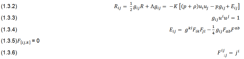
We choose the commoving co-ordinates so that
(1.3.7) u^1 〖=u〗^2=u^3 〖=0 and u〗^4=1/α
(1.3.7)
(1.3.7)
we label the co-ordinates (x, y, z, t) = ().
The off-diagonal components of (3.2.2) are
(1.3.8a)
(1.3.8b)
(1.3.8c)
(1.3.8d)
(1.3.8e)
(1.3.8f)
which lead to three possible cases :
- at least one of , non-zero. i.e., when the field is in X – direction only.
- at least one of , non-zero. i.e., when the field is in Y – direction only.
(iii) ,at least one of, non- zero. i.e., when the field is in Z – direction only.
Hence the electromagnetic field is non-null and consists of an electric and/or magnetic both of which are in the direction of same space axis. Without loss of generality, we may consider only case (i) in which the electric and magnetic field are in the X-direction.
we write
(1.3.9)
The diagonal components of the equation (1.3.2) may be written as
(1.3.10)
(1.3.11)
(1.3.12)
(1.3.13)
where the dot denotes the differentiation with respect to time t after the symbols. From these equations it is clear that are each functions of t alone.
From equation (1.3.5) and (1.3.9) it follows that is a constant and is a function of time t only i.e.
(1.3.14) =, =
where is a constant. In the case when = 0 which implies = 0, we get the model due to Roy and Prakash [24]. Here we assume that and find the only non vanishing components of to be
(1.3.15) =
Equation (1.3.15) shows that is space like, unless
where is a constant in which case = 0. The four-current is in general the sum of the convection current and conduction current (Licknerowicz [13] and Greenberg [10].
(1.3.16)
where the rest is charge density and is the conductivity. In the case consider here we have i.e. magneto-hydrodynamics. From equation (1.3.14) and (1.3.16) we find that conductivity is given by
(1.3.17)
where I = .
The requirement of positive conductivity in (1.3.17) puts further restrictions on. Hence in the Magnetohydrodynamics case metric function are restricted not only by field equations and energy condition (Hawking and Penrose [11]), they are also restricted by the requirement that the conductivity by positive for realistic model.
The equations (1.3.10-.1.3.13) are four equations in six unknown, , L. In order
to determine them, two more conditions have to impose on them. For this we assume that the space time is of degenerate Petrov type – I, the degeneracy being in y and z directions. This requires that . This condition is identically satisfied if. However, we shall take metric potentials to be unequal. We further assume that is such that
where is a constant.
From equation (1.3.12) and (1.3.13) we have
(1.3.18)
Equation (1.3.18) with condition gives
(1.3.19)
Since , equation (1.3.19) gives
(1.3.20)
From equation (1.3.11), (1.3.12) and (1.3.20) we have
(1.3.21)
Equation (1.3.18) on integration yields.
(1.3.22)
being an arbitrary constant of integration.
On putting and equation (1.3.22) goes to the form
(1.3.23) and equation (1.3.21) turns into
(1.3.24) =
From equation (1.3.23) and (1.3.24) we have
(1.3.25) = , which after the use of condition reduces to
(1.3.26)
Equation (1.3.26) on integration yields
(1.3.27) +
where is constant of integration from (1.3.23) and (1.3.27) we get
(1.3.28) where (1.3.29) =
Integration of (1.3.28) gives
(1.3.30)
where is constant of integration and
(1.3.31)
Hence we have
(1.3.32)
And (1.3.33)
Therefore the metric (1.3.1) can be written as
(1.3.34)
This by the use of equation (1.3.19), (1.3.26), (1.3.32) and (1.3.33) takes the form
(1.3.35)
The transformation
(1.3.36)
reduces (1.3.36) to the form (1.3.37)
where g , .
Again the use of transformation
leads (1.3.37) to the form.(1.3.38)
.
1.4 SOME PHYSICAL FEATURES:
(a). The distribution in the Model. :-
For the model (1.3.38) pressure p and density given by
(1.4.1) +
(1.4.2)
+
The model has to satisfy the reality conditions (Ellis [8]).
(i)
(ii)
This requires
(1.4.3) +
And (1.4.4) +
In the case of stiff matter ( = p).
(1.4.5) and (1.4.6)
The flow vector of the distribution is given by
(1.4.7)
Tensor of rotation defined by (1.4.8)
is identically zero. Thus the fluid filling the universe is non-rotational. The scalar of expansion is given by (1.4.9)
The component of the shear tensor defined by
(1.4.10)
are given by (1.4.11)
(1.4.12)
(1.4.13) 4.14)
. . .
The other component of are zero.
(b). The Doppler effect in the Model. :-
The track of light in the model (1.3.38) is given by setting
i.e,
(1.4.15) M + + =
For the case when velocity is along z-axis, eq. (1.4.15) gives
(1.4.16) = =
Hence the light pulse leaving a particle at (0, 0, z) at time T1 would arrive at a later time T2 given by
(1.4.17)
Hence
=
where = is the z – components of the velocity of the particle at the time of emission, and are the value of for and respectively. From the above equation we get
(1.4.18) =
The proper time interval between successive wave crests as measured by the local observer moving with the source is given by
(1.4.19) =
This can be written as
(1.4.20.i) =
where U is the velocity of source at the time of emission. Similarly we may write
(1.4.20.ii) =
As the proper time interval between the receptions of two successive wave crests by an observer at rest at the origin. Hence following Tolman [28] the red shift in this case is given by
(1.4.21)
= .
(c). Newtonian analogue of force in the Model. :-
Here we study the effect of electromagnetic field in force term (Narlikar and Singh [16]). It is well known that Christoffel three index symbols for the Riemannian metric of general relativity
defined by (1.4.22) =
and (1.4.23) are not tensor, but the difference of two such symbols of the same kind is a tensor. Thus if be Christoffel-index symbol for another metric
(1.4.24) ,
The difference (1.4.25) is a tensor.
The equation of the geodesies may now be cast in the form
(1.4.26) + =
In a region free from gravitation the geodesics are given by
(1.4.27) + =
Hence the gravitational effects depend only on the residual term . Since is arbitrary, the gravitational effects have to be associated with the tensor only. It can be seen that (Rosen [22]) (1.4.28) =
where commas ( , ) denotes co-variant differentiation with respect to Y-metric. A co-variant differentiation with respect to metric will be denoted by a semi colon ( ; ).
From (1.4.25) we have (1.4.29) =
If we write (1.4.30) =
Then and given by (1.4.28) and (1.4.29) are associated tensors.
The – tensor thus defined contain only the first order partial derivatives of the metric potential. Since – tensors are defined against the background of an arbitrary flat substratum; they would vary with the choice of the later for the same gravitational field. The importance of the ’s consists in the fact that the gravitational force of the Newtonian theory appears through them.
The vectors are defined as follow (Narlikar and Singh[16]).
(1.4.31) =
(1.4.32) = =
where.
For the line element (1.4.38), we have
(1.4.33)
and
(1.4.34)
(1.4.35)
The corresponding flat metric is taken to be that of special relativity
(1.4.36)
Thus,
(1.4.37) and (1.4.38)
From equation (3.2.35) and (3.2.38)
(1.4.39) = From (1.4.28) and (1.4.29) we get
(1.4.40) = and
(1.4.41) =
Thus we find that both are null force vectors. have no Newtonian analogues. In the absence of electromagnetic field (i.e. ) we see-
(1.4.42) =
(1.4.43) =
Also pressure and density are found in this case
(1.4.44)
(1.4.45) where is the value of when there is no electromagnetic field.
1.5 DISSCUSION :
Here in this chapter, considering the cylindrically symmetric metric of Marder [14]. We have constructed a non static spatially homogeneous Petrov type -I cosmological model assuming the energy momentum tensor to be that of a perfect fluid with an electromagnetic field and the four current is either zero or space like. The requirement that the conductivity be positive imposes an additional condition on the metric functions. It is seen that when m = 1, then our metric is undefined. We have calculated various physical and geometrical properties e.g. pressure, density, rotation scalar of expansion and components of shear tensor. We have also discussed Doppler Effect and a Newtonian analogue of force in the model. It is observed that when the cosmological constant ᴧ= 0, then in the absence of electromagnetic field pressure and density becomes equal and conversely if pressure and density are equal there is no electromagnetic field.
1.6 REFERENCES :
[1] Bali, R., Jain, D. R. (1990): Astrophysics and Space Science, 175, 89.
[2] Bergman, M.S. (1991): Phys. Rev., D43, 1075.
[3] Bali, R. and Yadav, M.K. (2005): Pramana., Journ. Phys., 64,187.
[4] Casama, R., Meloc. Pimentel B., (2006): Astrophys.Space. Sci., 305, 125.
[5] Cowling, T.G. (1945): M.N., 105, 166.
[6] Cowling, T.G. (1957): Magneto-hydrodynamics, Inter Science Publication, 10, 132.
[7] De, U.K. (1975): Acta. Phys. Polon., B6, 341.
[8] Ellis, G.F.R. (1971): General Relativity and Cosmology; Ed. Sach, R.K.,
Academic Press, New York, 104.
[9] Grareeki, J. (1995): G.R.G., 27,55.
[10] Greenberg, P.J. (1971): Astrophysics J., 164, 589.
[11] Hawking, S.W. and Penrose, R. (1973): The large Scale Structure of
Space time, Cambridge University Press, London.
[12] Jacobs, K.C. (1967): Astrophys. J., 153, 661.
[12a] Jacobs, K.C. (1969) : Astrophys. J., 155, 379.
[13] Liknerowicz, A. (1967) : Relativistic Hydrodynamics and Magneto-
Hydrodynamics, Benjamin, New York, Chap., 4.
[14] Marder, L. (1958): Proc. R. Soc., A246, 133.
[15] Manoghan, J.J. (1966): Mon. Not. Roy. Astron. Soc. (G.B.), 134, 275.
[16] Narlikar, V.V. and Singh, K.P. (1951): Proc. Nat. Inst. Science(India), 17, 31.
[17] Paul, B.B. (2003) : Pramana Journ. Phys., 61, 1055.
[18] Paul, B.B. (2000) : Ind. J. Pure Appl. Math.,31, 305.
[19] Pradhan, A. and Vishwakarma, A.K. (2002): Ind. J. Pure Appl. Math.,
33, 1239.
[20] Pradhan,A.,H. Amirhaschi., et.al. (2011):Int.J.Theo,Phys.,50, 56.
[21] Rendal, A.D. (1995): G.R.G. 27.,213.
[22] Rosen, N. (1940): Phys. Rev., 57, 147.
[23] Rao, V.U.M.,Vinutha.T.,et.al. (2008): Astrophys. Space. Sci., 314, 213.
[24] Roy, S.R. and Prakash, S. (1978): Indian J. Phys., 52B, 47.
[25] Shikin, I.S. (1996) : Dokl. Akad. Nauk, S.S.S.R., 171, 73.
[26] Singh, T. and Yadav, R.B.S. (1980) : Indian J. Pure Appl. Math., 11(7),
917.
[27] Thorne, K.S. (1967): Astrophys. J., 148, 51.
[28] Tolman, R.C. (1962): Relativity, Thermodynamics and Cosmology, Oxford University Press, 289.
[29] Tupper, B.O.J. (1977a): Phys. Rev. D., 15, 2153.
[30] Tupper, B.O.J. (1977b): Astrophys. J., 216, 192.
[31] Wrubel, M.N. (1952) : Astrophs. J., 116, 193.
[32] Yadav, R.B.S. and Singh, R. (1997): Math. Ed., 31, 215.
[33] Yadav, R.B.S. and Purushottam (2004): Acta. Sci. Ind., 30,629.
[34] Zeldovich, Ya. Ba. (1965): Zh. Exper. Teor. Fiz. (U.S.S.R.)., 48, 986.
[35] Zeldovich, Ya. B. and Novikov. I.D. (1971): Relativistic Astrophys., Vol.-1., The Univ. Of Chicago Press, 459.
[36] Zeldovich, Ya. B., Ruzimainkin, A., Sokoloff, D., Magnetic field (1993):
Astrophysics (Gordon and Breach, New York).
[37] ZIA, R., Singh R.P. (2012): Rom Journ. Phys., Vol. -57, No.- 3-4, P.g.- 761-778.