|
Chaos & Logistic Maps
We live in a nonlinear world. The evolution of real life systems is intrinsically nonlinear. The analysis of nonlinear systems is hard and complex but one can’t do without that. The lack of periodicity and certainty are common in natural phenomena. They are often unpredictable, despite their simplicity and determinism. They exhibit chaotic behavior. For systems with bounded solutions, it is found that non-periodic solutions are ordinarily unstable with small modifications so that slightly differing initial states can evolve into considerably different states. They are said to be sensitive to the initial conditions of the system. They possess constrained numerical solutions. Solutions of these systems can be best visualized with trajectories in phase space. To be concise- sensitivity, determinism and nonlinearity (or recurrence)- are three simple constraints of chaos.
1. Introduction
Chaos implies an irregular, seemingly random change in time or motion which is too complex to predict in detail or rather compute with any given precision in the long run. We say ‘seemingly’ random because the physical laws and the forces that govern the motion are all perfectly deterministic and given. The name Chaos Theory comes from the fact that systems which the theory describes are apparently disordered and indiscipline. Formally, chaos theory is defined as the study of complex nonlinear dynamic systems. A system is complex if there is something more to say about it. Nonlinear implies recursion and higher mathematical algorithms and dynamic implies non-constant and non-periodic. The first incident of chaos was noticed, accidentally, by Edward N. Lorenz, a meteorologist at Massachusetts Institute of Technology, in 1960’s and the chaos theory had its birth then. The term ‘chaos’ was coined by Li and Yorke in 1975. Chaos bears a very delicate bond with the initial conditions of a system. This hypersensitivity to initial conditions came to be known as the Butterfly Effect. Lorenz in one of his address exclaimed-‘The flap of a butterfly’s wings in Brazil sets off a tornado in Texas’. It clearly epitomizes chaos today. Conceiving this idea, Lorenz stated that it is impossible to predict the weather accurately. |
|
Thus sensitivity, determinism and nonlinearity are three simple constraints of chaos. Any system having these constraints will, surely, go chaotic-be it small (simple), large (complex), conservative or dissipative-for given initial conditions at certain threshold values of control parameter(s). It must be noted that all complex systems are not chaotic but all chaotic systems are, indeed, complex. Complex systems invariably involve nonlinearity and are sensitive to initial conditions. Chaos is a ‘condition’ which when only furnished with, the system results in unpredictability and strange behavior.
Logistic Equation & Mappings
Logistic map is an important classical problem of chaotic dynamics. This has become something of a poor man’s laboratory to gain hands-on experience with chaos. The logistic map is a difference equation of the form Xn+1=f(k,Xn) , Xn lying in [0 1]. It gives the evolution of a variable X as function ‘f’ of discretised time ‘n’. We choose the initial value X0 and then a set of X’s is generated which when plotted in the phase space gives a trajectory. Here, k is a control parameter which, of course, can be tuned. Varying the parameter k leads to the onset of chaotic behavior through the mechanism of bifurcation. It seems logical to suppose that as the control parameter is raised, the lower dimensional attractors get destabilized in favor of the higher dimensional attractors which eventually lead to chaos.
6.1 Verhulst-May Logistic Map
The difference equation , Xn+1=kXn(1-Xn), is called the logistic map. The logistic map is the discrete version of the corresponding continuous differential equation given by P.F Verhulst in 1845. He had used it to model population growth subject to limited resources (or logistics). Hence, the qualifier ‘logistic’. The discrete version of the logistic map was studied extensively by the physicist turned ecologist-biologist Robert May in 1976. In his words- ‘Not only in research but in the everyday world of politics and economics, we would be better off if more people realized that simple systems do not necessarily possess simple dynamic properties’. |
For control parameter k=2, a difference of 0.0000001 in seed values results in two different trajectories. This shows sensitive dependence on initial conditions.
Characteristics of Logistic Map, Xn+1=kXn(1-Xn)
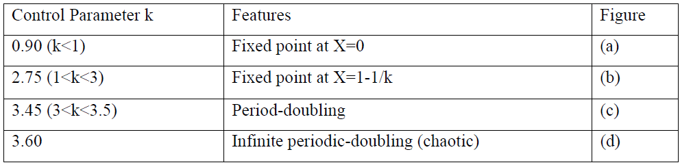
F(X)=k*X(1-X)
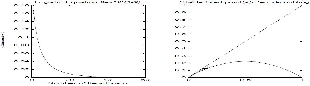
(a) For k=0.90
For seed value X0=0.25
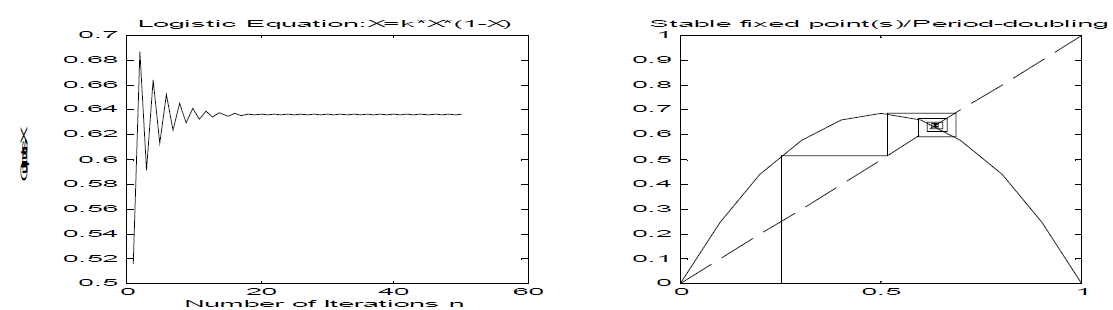
(b) For k=2.75
For seed value X0=0.25 02040600.50.520.540.560.580.60.620.640.660.680.7Number of
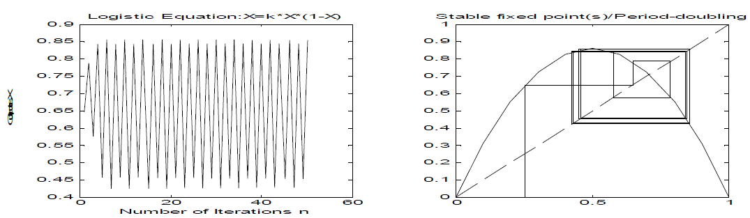
(c) For k=3.45
For seed value X0=0.25
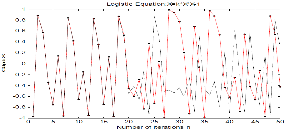
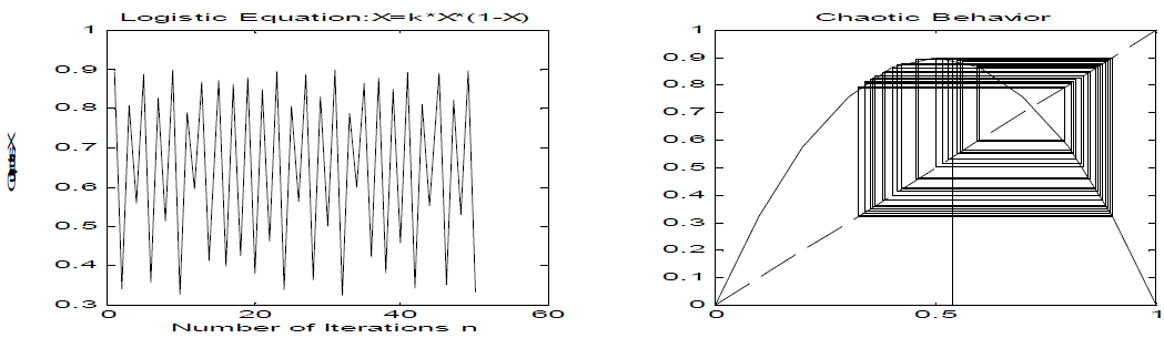
(d) For k=3.60
For seed value X0=0.25
For seed value X0=0.54
For seed value X0=0.86
Results
We explored the outputs of different functions with varying values of control parameter and seed values and obtained graphical outputs.
Acknowledgement
I am grateful to Prof. (Dr.) Vijay A. Singh, HBCSE (TIFR).
References
(1) Kumar, N. (1996). Deterministic Chaos: Complex Chance Out of Simple Necessity. Universities Press (India) Limited, Hyderabad.
(2) Verma, R.C., Ahluwalia, P.K., and Sharma, K.C. Computational Physics: An Introduction. New Age International Publishers, New Delhi.
(3) Smith, Leonard A. (2007). CHAOS: A Very Short Introduction, 1st ed. Oxford University Press, New York. (4) Pratap, Rudra (2006). Getting Started With MATLAB 7: A Quick Introduction for Scientists and Engineers. Oxford University Press, New York.
|